Quick note on Normalising flow for SBI
Normalising flow is commonly used for density estimation in generative model. It is also used in Simulatoin-Based Inference (SBI) to estimate conditional density. Specifically, \(p(\theta | \mathcal{D})\) for neural posterior estimation (NPE) and \(p(\mathcal{D} | \theta)\) for neural likelihood estimation (NLE). In this post, I will quickly explain how normalizing flow can estimate density with some focus on the application in SBI.
In generative model we are interested in estimating distribution of \(x \in \mathbb{R}^D\) by integrating out latent variable \(z \in \mathbb{R}^D\), that is
\[ p(x) = \int p(x | z)p_z(z)dz \]
The integral is usually intractable. In normalizing flow, we pick \(p_z(z)\) to be a simple distirbution such as standard normal distribution \(N(0, I_D)\), and transform \(p_z(z)\) with \(g: \mathbb{R}^D \rightarrow \mathbb{R}^D\). We pick \(g\) to be diffeomorphism, that is, \(g\) is 1. bijective, 2. differentiable, 3. its inverse is differentiable. This allows us to express \(p(x)\) using change of variable formula (without any intractable integral involved)
\[ p(x) = p_z(g^{-1}(x)) \left|\det \frac{\partial g^{-1}(x)}{\partial x} \right| := p_z(f(x)) \left|\det \frac{\partial f(x)}{\partial x} \right| \] We just defined \(f := g^{-1}\). \(g\) is referred as generative path because we try to generate \(x\) from a simple distribution \(p_z\), whereas \(f\) is referred as normalising path because we try to degenerate \(x\) back to \(z \sim p_z\), where \(p_z\) is usually normal distribution.
\(f\) is usually parameterized by neural network to maximise likelihood \(p(x)\). \(f\) is usually chosen such that the determinant of the Jacobian is easy to calculate. Training and evaluation of density requires normalising path while sampling requires generative path as
\[ x \sim p(x) \mathrel{\Leftrightarrow} z \sim p_z(z), x = g(z) \]
People often care about \(f\) because fast evaluation of \(f\) is needed for fast training. If we need fast sampling, then \(g\) is cared.
In SBI, coupling flow and autoregressive flow is commonly used.
Coupling flow
\[ \begin{align} x &= [x^A, x^B] \\ \phi &= NN(x^B) \\ y^A &= \mathbf{h}_\phi(x^A) = [h_{\phi_1}(x_1),...,h_{\phi_d}(x_d)] \\ y^B &= x^B \\ y &= [y^A, y^B] \end{align} \]
Firstly, \(x\) is split into two dimension such that \(x^A \in \mathbb{R}^d, x^B \in \mathbb{R}^{D - d}\). Then one part is fed into NN: \(\mathbb{R}^{D - d} \rightarrow \mathbb{R}^k\) to learn parameter \(\phi \in \mathbb{R}^k\). The NN is referred as conditioner. This \(\phi\) is then coupled with another part \(x^A\) through invertible and differentiable function \(\mathbf{h}\) called transformer or coupling function. \(k\) depends on the choice of coupling function. Note that transformer is nothing to do with the ‘query-key-value’ transformers. Coupling function is usually applied element-wise. This transformed \(x^A\) is then concatenated with \(x^B\), which gives output \(y\). Its inverse is given by
\[ \begin{align} x^B &= y^B \\ \phi &= NN(x^B) \\ x^A & = \mathbf{h}_{\phi}^{-1}(y^A) \end{align} \]
This ‘coupling’ is repeated multiple times, combined with non-stochastic permutation such that all the dimensions \(i = 1,...,D\) are interacted to each other. The determinant of Jacobian is given by \(\prod_{i=1}^d \frac{\partial h_{\phi_i}(x_i)}{\partial x_i}\).
In NPE, \(x \leftarrow \theta\) and the conditioner is also conditioned on data as \(\phi = NN(\theta^B, \mathcal{D})\). In NLE, \(x \leftarrow \mathcal{D}\) and \(\phi = NN(\mathcal{D}^B, \theta)\)
Autoregressive flow
\[ \begin{align} \text{For } i &= 2,...,D:\\ \phi_i &= NN(x_{1:i-1}) \\ y_i &= h_{\phi_i}(x_i)\\ \end{align} \]
where \(\phi_1\) is constant. This is very similar to coupling flow except that instead of splitting dimensions into half, dimension is split in autoregressive manners into \(x_i\) and \(x_{1:i-1}\) mutiple times. In practice, this coupling functions can be implemented without recursion using masking.
In NPE, \(\phi_1 = NN(\mathcal{D}), \phi_i = NN(\theta_{1:i-1}, \mathcal{D}), 1 < i \leq D\). In NLE, \(\phi_1 = NN(\theta),\phi_i = NN(\mathcal{D}_{1:i-1}, \theta), 1 < i \leq D\)
Coupling function
Affine
\[ h_{\phi_{i}}(x_i) = \alpha_i x_i + \beta_i, \quad \phi_i = (\alpha_i, \beta_i) \]
where \(\alpha_i > 0, \beta_i \in \mathbb{R}\). For affine coupling function, \(k = d \times 2\).
Monotonic rational quadratic spline
In neural spline flow, monotonic rational quadratic spline (RQ-spline) is used for \(h\). It allows to model more expressive transformation from \(x\) to \(y\) and to \(z\) at final. Monotonicity is necessary for bijectivity. In a nutshell, \(h\) is defined in the interval \([-B, B]\) and that interval is split into \(K\) bins using \(K + 1\) knots, where \(B\) and \(K\) are hyper-parameters. The height and the width of the bins are trainable parameters \((\phi_{h,j}, \phi_{w, j}), j = 1,...,K\), and derivatives at each knots are also trainable parameters \(\phi_{d,j}, j = 1,...,K-1\). These parameters defines the RQ-spline. In total, the coupling function have \(k = (3K - 1) \times d\) parameters.
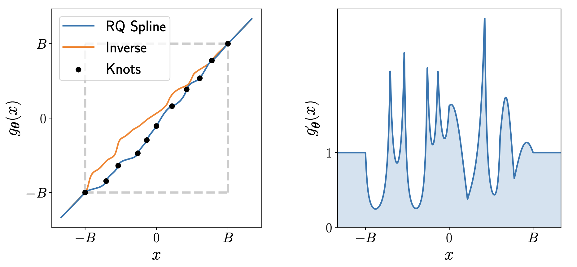
In this figure, \(K = 10\) is picked.
Bibliography
[1] I. Kobyzev, S. J. D. Prince and M. A. Brubaker, “Normalizing Flows: An Introduction and Review of Current Methods,” in IEEE Transactions on Pattern Analysis and Machine Intelligence, vol. 43, no. 11, pp. 3964-3979.
[2] Durkan, C., Bekasov, A., Murray, I., & Papamakarios, G. (2019). Neural Spline Flows. Advances in Neural Information Processing Systems, abs/1906.04032. https://proceedings.neurips.cc/paper/2019/hash/7ac71d433f282034e088473244df8c02-Abstract.html
[3] Radev, S. T., Mertens, U. K., Voss, A., Ardizzone, L., & Kothe, U. (2022). BayesFlow: Learning Complex Stochastic Models With Invertible Neural Networks. IEEE Transactions on Neural Networks and Learning Systems, 33(4), 1452–1466.
Appendix
Dual coupling
Sometimes, one block of coupling is defined as two coupling as in [3] such that both split is transformed by coupling function in one unit of coupling.
\[ \begin{align} x &= [x^A, x^B] \\ \phi_1 &= NN_1(x^B) \\ y^A &= \mathbf{h}_{\phi_1}(x^A) \\ \phi_2 &= NN_2(y^A)\\ y^B &= \mathbf{h}_{\phi_2}(x^B) \\ y &= [y^A, y^B] \end{align} \]
This is same as applying single coupling flow followed by permutation, which swap \(x^A\) and \(x^B\) and applying another coupling flow.
When \(D = 1\)
In generative model \(x\) is usually something high dimensional like image. But in SBI, \(D\) could be 1. Coupling flow could be applied in such case. For example in NPE, if \(\theta \in \mathbb{R}\) and consider only one coupling, then we have
\[ \begin{align} \phi &= NN(\mathcal{D}) \\ z &= \mathbf{h}_{\phi}(\theta) \end{align} \]
In this case, \(\theta\) is not going to be coupled with another split of \(\theta\) because \(\theta\) is just one-dimensional, but it is still coupled with \(\mathcal{D}\).
In this case, naturally, coupling flow is same as autoregressive flow given same conditioner and coupling function.